
One of the main functionalities of Orbit is to classify different structures in your image, e.g. tissue classes. This could be used to quantify the amount of stained tissue vs. the whole tissue.
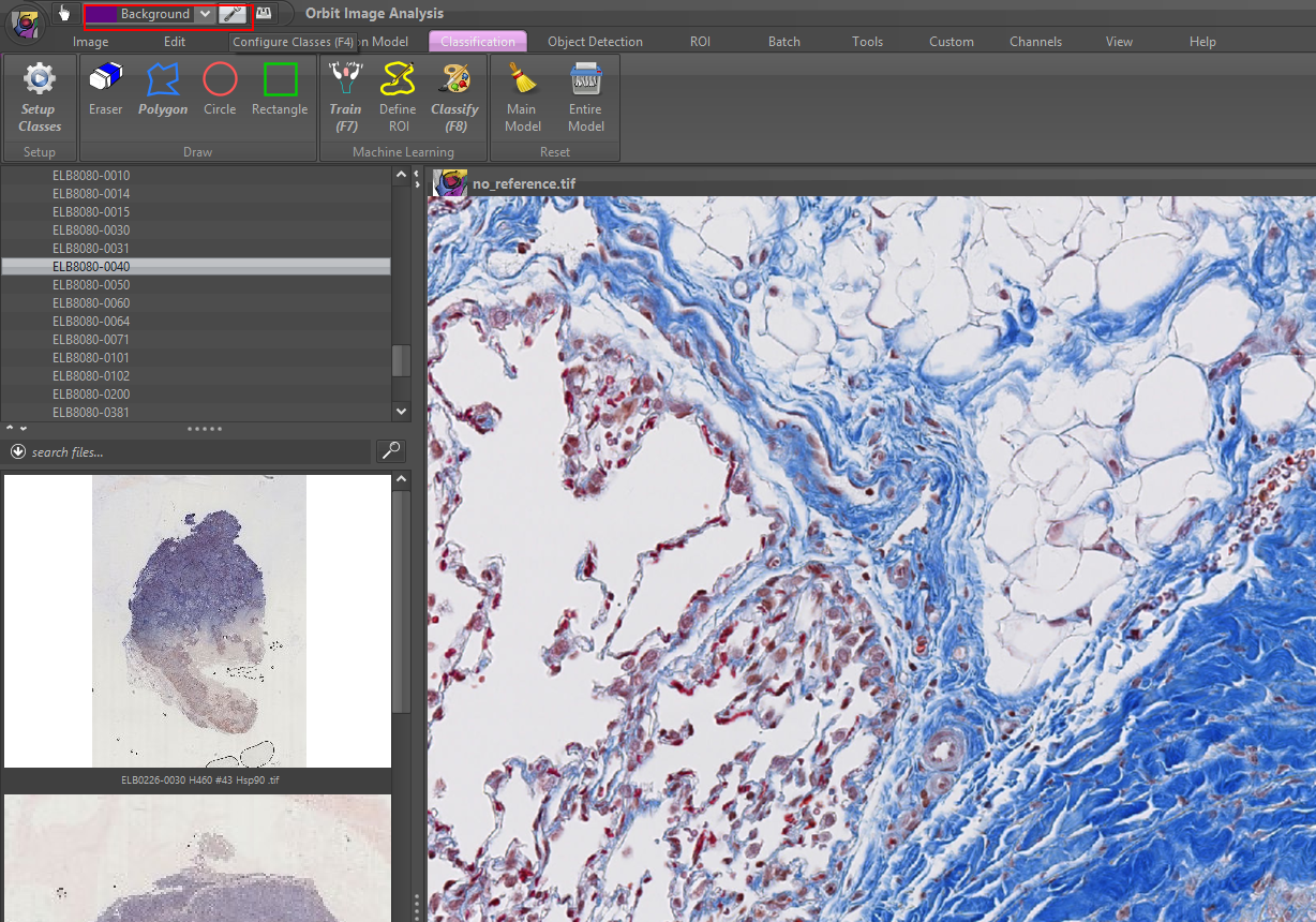
For (e.g. tissue) classification, first we select the classification tab. If you did s.th. before you can click on ‘setup classes’ to setup the classes for a classification, which is by default the case.
Btw: a general procedure in Orbit is to select a task represented by the tabs and then work the buttons from left to right. Mouse over a button to get some help what to do.
1) Open an image and setup your tissue classes (you can use the shortcut F4 to open the class setup).
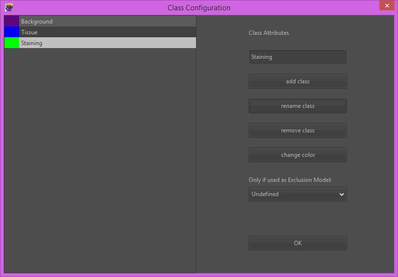
2) Define your classes, e.g. Background, Tissue, Staining. You can specify an arbitrary number of classes.
To rename a class of change it’s color, first select the class, then press rename or change the color. It is helpful to chose a class color which is the counter-color to the real class color in the image, so that you see your drawings inside that class later.
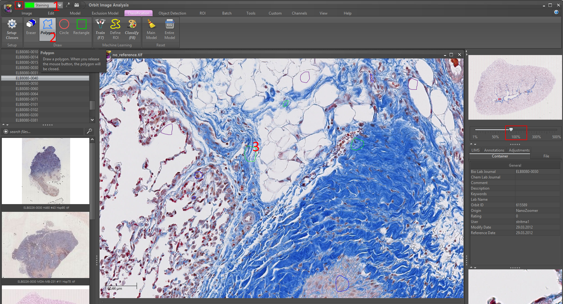
3) For each class, first select the class from the class-dropdown, then select a drawing tool (e.g. polygon) and draw some small example regions in your image.
The idea here is to ‘show’ Orbit representative regions for each tissue class. Representative here means the whole variability, so mark some of the brightest and some of the darkest parts of each class. You can also open several images and mark classes on several images, e.g. if you have one brighter and one darker image containing the same tissue class. In most cases 3-5 small regions per class are sufficient.
Draw the class regions at a magnification of around 100% (top-right side scale slider) because this is also the resolution on which the computer ‘sees’ your image.
You can press ‘space’ while drawing to get a temporary hand tool to move your image. Press F6 when in drawing mode to get the hand tool back or click on the hand tool icon in the menu bar top left.
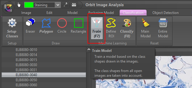
4) Click on the Train (F7) to train your model based on your class regions. You should see a progress bar on the right which disappears when the training is complete.
Optional: open the log (Help -> view log) to see the accuracy of your model with respect to your training regions. (And then go back to the classification tab.)
5) Use the Region of Interest (ROI) tool to define a ROI in your image where you want to test the classification model. For small images you can classify without a ROI, then the whole image will be classified.
It is strongly recommended to set the scale (top-right scale bar) at around 100% magnification. (Otherwise it might be very slow.)
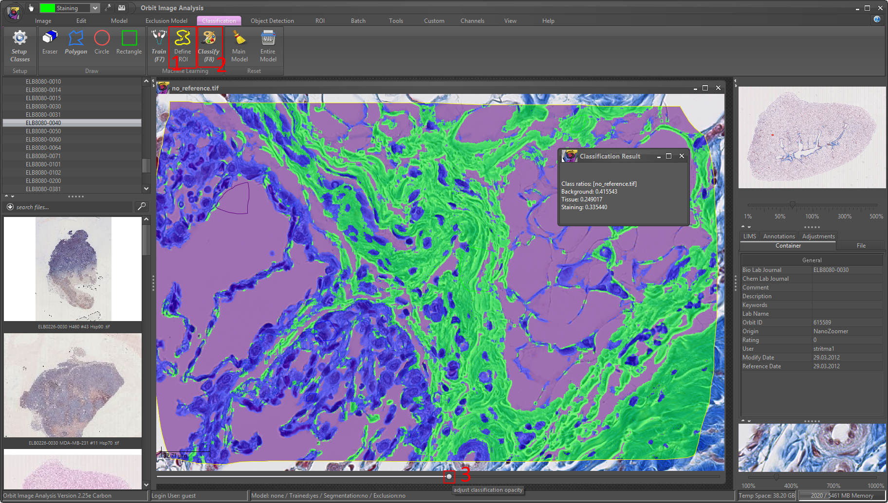
Then click on Classify (F8) to classify the ROI of your image. You’ll see a popup which shows you the ratios per class. As you can see they sum up to one, thus you can multiply them with 100 to get percentage values.
6) Visually validate the results. Use the bottom slider of your image and drag it to the right to see the classification map. If you’re happy with the result you can classify the whole image (reset the ROI with ROI -> reset).
If your not fine with the results iteratively improve your model by drawing more training regions or removing some (step 3).
Congratulation, you did your fist tissue classification!
Hint: Press F3 to open the feature configuration dialog. Change the structure size to values between 0 and 10, click on train and classify again, and see what happens. The structure size defines if Orbit looks more on fine grained structures (low values) or on the larger context (high values). See the triangle example in the handbook for more details about that.
What you created by drawing class regions and training is called a model. This model can be saved to disk or in Orbit (Model -> Save…) and reused to quantify a set of images. To apply the model to a set of images use the Batch -> Local Execution (or Scaleout Execution if you have a Spark cluster).